Learning TensorFlow via a 3D printing Project
This is a slightly cleaned up version of the slides for a presentation I gave at the SLCPy meetup a while ago. I intended to write something with nice prose and turn it into something that can stand on its own without the verbal commentary that went along with it, but that isn't going to happen so here are the raw slides.
There is a video of the event but unfortunately because of technical troubles it is audio only. Despite the title of the video the meetup happened in March. The first hour of the video is just people talking eating pizza and random pieces of business for the python group. Skip to 1 hour and 18 minutes in to the video to hear the actual presentation.
from IPython.display import Image
What is TensorFlow
-
TensorFlow is Google's open source Python library for machine learning.
-
TensorFlow is a way to take advantage of GPU's and multiple core CPU's for heavy number crunching.
-
TensorFlow is a solution to remove the overhead of returning to the python interpreter in between each step of a heavy numerical code.
What is Machine Learning?
My Definition: Machine learning is declarative programming taken to its logical extreme.
Declarative Programming: Tell a computer what we want but not exactly how to do it.
Supervised Machine Learning: Tell a computer what we want (a metric) and let it figure out how to do it (best parameters for our function).
How To Learn TensorFlow
Look at some tutorials and get one working.
-
Getting Started Including MNIST hello world. https://www.tensorflow.org/get_started/get_started
-
Mandelbrot Set Computation https://www.tensorflow.org/tutorials/mandelbrot
-
Transfer Learning by Retraining Last Layer of Inception https://www.tensorflow.org/tutorials/image_retraining
Then pick your own project and do it!
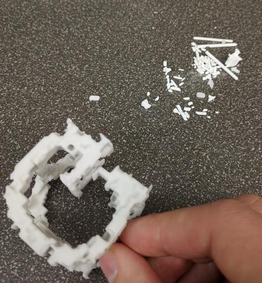
I vowed to use the 3D printing capabilities on campus at least once before I leave the U. Why not kill two birds with one stone? Learn tesor flow by making it learn to 3D print!
But 3D Printing is Not a Machine Learning Problem! Right?
- If we can tell a computer how to represent a 3D object as a big pile of numbers... (parameters)
- and we can tell a computer how to compute a numerical "desirability" of those objects... (a metric)
3D Printing Can Be A Machine Learning Problem!
- If we can tell a computer how to represent an object we would like as a big pile of numbers...
- and we can tell a computer how to compute a numerical "desirability" of those objects...
Then we can use the tools of machine learning to "learn" a representation for our object!
TensorFlow Overview
-
tf.Operation --> nodes in an execution graph
-
tf.Tensor --> outputs of operations
-
tf.Variable --> free parameters
-
tf.placeholder --> data and/or hyper parameters
-
tf.Session --> manages state of Variables and executes operations on Tensors
Analogy To Mathematical Function Optimization
In the familar mathematical context of model fitting we might write.
$$ {\large y = f(x | \theta)} $$Where we wish to tweak the parameters $\theta$ to minimize some risk $R$ given observations $x_{obs}$ and $y_{obs}$ The correspondence in tensor flow is fairly one to one
- y, x <--> tf.placeholder
- f, R<--> tf.Operation
- $\theta$ <--> tf.Variable
The Hammer: Mini-Batch Stochastic Gradient Descent
- calculate the derivative of our metric with respect to our current parameters for some small batch of data.
- Then move "down the slope" by some small step size (the learning rate).
- Easy GPU/Multi-Core Number Crunching.
- Auto-differentiation
- Auto-differentiation
- Auto-differentiation
When you have millions of parameters and function evaluations can take seconds estimating $\partial f(x | \theta)/ \partial \theta_i$ for all million parameters using a finite differences method is not feasible.
You need an analytic form for the derivative.
TensorFlow is not the only thing that does this (e.g. STAN, and Theano) just the newest slickest thing that does it.
Baby Steps: Fit A Linear Model
import numpy as np
import matplotlib.pyplot as plt
%matplotlib inline
plt.rcParams.update({"figure.figsize":(12,6), "font.size":16})
np.random.seed(4321)
true_slope = np.e
true_offset = np.pi
#make some noisy data
npts = 50
x = np.random.uniform(0, 1, npts)
noise = np.random.standard_cauchy(size=(npts,))
y_true = true_slope*x + true_offset
y = y_true + noise
plt.scatter(x, y)
xspan = np.linspace(0, 1, 100)
lsq_soln = np.linalg.lstsq(np.vander(x, 2), y)[0]
lsq_model = np.dot(np.vander(xspan, 2), lsq_soln)
plt.plot(xspan, xspan*true_slope + true_offset, c="k", lw=3, alpha=0.8, label="True")
plt.plot(xspan, lsq_model, c="r", lw=3, label="Least Squares")
plt.xlabel("measured x")
plt.ylabel("measured y")
import tensorflow as tf
#TensorFlow is still rapidly evolving so the version you are using really matters
print("TensorFlow version", tf.__version__)
TensorFlow Model
slope = tf.Variable(0.0, dtype=tf.float32)
offset = tf.Variable(0.0, dtype=tf.float32)
batch_size = 15
x_placeholder = tf.placeholder(dtype=tf.float32, shape=(batch_size,))
y_placeholder = tf.placeholder(dtype=tf.float32, shape=(batch_size,))
f = slope*x_placeholder + offset
sq_sum = tf.reduce_sum((y_placeholder - f)**2)
Training Operation
opt = tf.train.GradientDescentOptimizer(learning_rate=0.01)
train_op = opt.minimize(sq_sum)
Learning
param_history = []
batch_history = []
with tf.Session() as sess: #context manager for the session
init_op = tf.global_variables_initializer()
sess.run(init_op)
n_batch = 20
iter_per_batch = 10
for batch_idx in range(n_batch):
#get a batch of data
batch_idxs = np.random.random(npts).argsort()[:batch_size]
x_batch = x[batch_idxs]
y_batch = y[batch_idxs]
batch_history.append(batch_idxs)
for iter_idx in range(iter_per_batch):
#train our model
sess.run(train_op, feed_dict={x_placeholder:x_batch, y_placeholder:y_batch})
param_history.append(sess.run([slope, offset]))
param_history = np.array(param_history)
Training Path
plt.plot(*param_history.T, zorder=0, c="k", lw=2)
plt.scatter(*param_history.T, c=np.arange(len(param_history)), s=80, cmap="viridis")
cbar = plt.colorbar()
cbar.set_label("Iteration")
plt.axvline(true_slope, c="r", label="True Values")
plt.axhline(true_offset, c="r", )
plt.axvline(lsq_soln[0], label="Least Squares")
plt.axhline(lsq_soln[1])
plt.xlabel("Estimated Slope")
plt.ylabel("Etimated Offset")
Inspiration
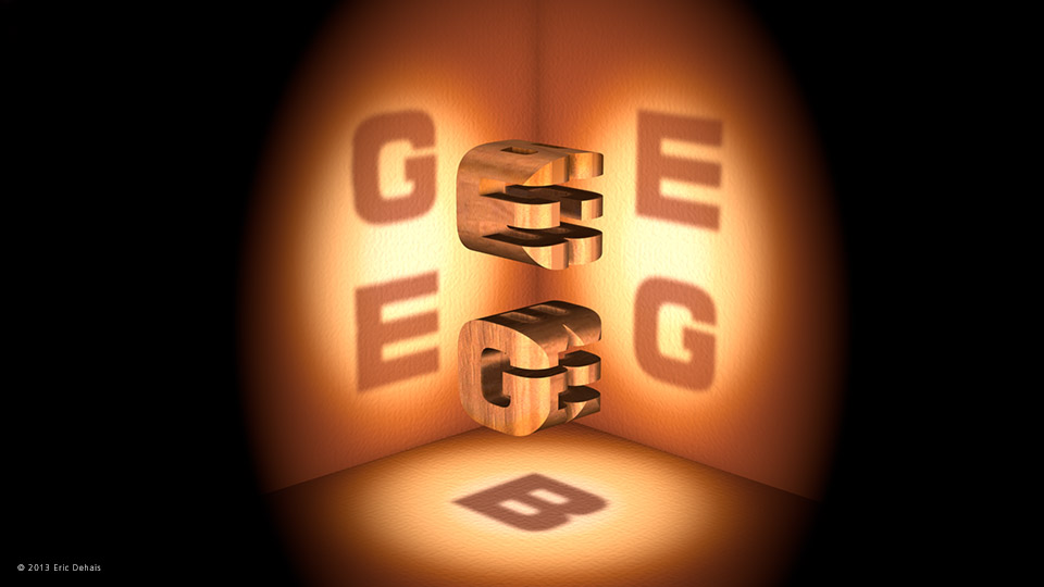
General Strategy
- Represent objects in TensorFlow as point clouds
- Evaluate silhouettes of ojbects from each desired perspective.
- Compare the silhouette to a desired image.
- Calculate the sum of squared residuals of actual to desired silhouettes
- Use TensorFlow to optimize!
- Turn point cloud into mesh using the marching cubes algorithm.
Why a Point Cloud? Wouldn't a 3D Tensor Be Better?
- More physically Intuitive
- (No) grid edges.
- Easier to effectively visualize
- More adaptive representation (sparse + easily refinable)
- Better illustrates the sort of troubles encountered in deep learning e.g.
- Many local optima
- Co-adaptation of parameters
- Vanishing derivatives problem
- Also I just like point clouds.
Calculating a Silhouette
def make_coordinate_sampler(x, lower_bound, upper_bound, npts):
cx =(npts-1)*(x-lower_bound)/(upper_bound-lower_bound)
nearest_xi_float = tf.floor(cx+0.5)
nearest_xi_int = tf.to_int64(nearest_xi_float)
delta = cx-nearest_xi_float
return {
"continuous_index":cx,
"nearest_index":nearest_xi_int,
"delta":delta,
}
def make_silhouette(
x, y,
bounds,
npts,
silhouette_shape,
delta_footprint,
radial_basis_function,
):
nx, ny = silhouette_shape
min_x, max_x, min_y, max_y = bounds
x_sampler = make_coordinate_sampler(x, min_x, max_x, nx)
y_sampler = make_coordinate_sampler(y, min_y, max_y, ny)
point_indexes = []
x_indexes = []
y_indexes = []
footprint_indexes = []
rbf_weights = []
n_foot = len(delta_footprint)
for footprint_idx in range(n_foot):
dx, dy = delta_footprint[footprint_idx]
x_idx = tf.clip_by_value(x_sampler["nearest_index"] - dx, 0, nx-1)
y_idx = tf.clip_by_value(y_sampler["nearest_index"] - dy, 0, ny-1)
r_delta = tf.sqrt((x_sampler["delta"] + dx)**2 + (y_sampler["delta"] + dy)**2)
weight = radial_basis_function(r_delta)
rbf_weights.append(weight)
point_indexes.append(tf.range(0, npts, dtype=tf.int64))
x_indexes.append(x_idx)
y_indexes.append(y_idx)
footprint_indexes.append(tf.constant(np.repeat(footprint_idx, npts)))
#join the tensors together
rbf_weights = tf.concat(concat_dim=0, values=rbf_weights)
point_indexes = tf.concat(concat_dim=0, values=point_indexes)
x_indexes = tf.concat(concat_dim=0, values=x_indexes)
y_indexes = tf.concat(concat_dim=0, values=y_indexes)
footprint_indexes = tf.concat(concat_dim=0, values=footprint_indexes)
packed_indices = tf.stack([footprint_indexes, point_indexes, x_indexes, y_indexes], axis=1)
sparse_shape = tf.constant(np.array([n_foot, npts, nx, ny]))
sparse_opacity = tf.SparseTensor(packed_indices, values=rbf_weights, shape=sparse_shape)
#sum over the footprint and point indexes to get a 2D tensor
#dense_opacity = tf.sparse_reduce_sum(tf.sparse_reduce_sum_sparse(sparse_opacity, axis=0), axis=0)
dense_opacity = tf.reduce_sum(tf.sparse_reduce_sum(sparse_opacity, axis=1), axis=0)
silhouette = 1.0 - tf.exp(-0.5*tf.sqrt(dense_opacity))
return{
"silhouette":silhouette,
"opacity":dense_opacity,
}
import scipy.misc
def load_im(fname):
im = scipy.misc.imread(fname).astype(np.float32)
im /= np.max(im)
return im
G_im = load_im("G.jpg")
E_im = load_im("E.jpg")
B_im = load_im("B.jpg")
fig, ax = plt.subplots(1, 3)
for i, im in enumerate([G_im, E_im, B_im]):
ax[i].imshow(im, cmap="afmhot_r")
npts_cloud = 30000
init_cloud_positions = np.random.uniform(low=-1, high=1, size=(npts_cloud, 3)).astype(np.float32)
cloud = tf.Variable(init_cloud_positions, name="cloud")
def make_delta_footprint(n_delt, max_radius=2):
deltas = []
for dx in range(-n_delt, n_delt+1):
for dy in range(-n_delt, n_delt+1):
if np.sqrt(dx**2 + dy**2) < max_radius:
deltas.append((dx, dy))
return deltas
deltas = make_delta_footprint(2)
g_silhouette = make_silhouette(
x=cloud[:, 0],
y=cloud[:, 1],
bounds=(-1, 1, -1, 1),
npts=npts_cloud,
silhouette_shape=G_im.shape,
delta_footprint=deltas,
radial_basis_function = lambda r: tf.exp(-r**2),
)
e_silhouette = make_silhouette(
x=cloud[:, 0],
y=cloud[:, 2],
bounds=(-1, 1, -1, 1),
npts=npts_cloud,
silhouette_shape=E_im.shape,
delta_footprint=deltas,
radial_basis_function = lambda r: tf.exp(-r**2),
)
b_silhouette = make_silhouette(
x=cloud[:, 1],
y=cloud[:, 2],
bounds=(-1, 1, -1, 1),
npts=npts_cloud,
silhouette_shape=B_im.shape,
delta_footprint=deltas,
radial_basis_function = lambda r: tf.exp(-r**2),
)
g_resids = g_silhouette["silhouette"] - G_im
e_resids = e_silhouette["silhouette"] - E_im
b_resids = b_silhouette["silhouette"] - B_im
gsum = tf.reduce_sum(g_resids**2)
esum = tf.reduce_sum(e_resids**2)
bsum = tf.reduce_sum(b_resids**2)
resid_sq_sum = gsum + esum + bsum
learning_rate = tf.placeholder(dtype=tf.float32)
optimizer = tf.train.GradientDescentOptimizer(learning_rate=learning_rate)
global_step = tf.Variable(0, name='global_step', trainable=False)
train_op = optimizer.minimize(resid_sq_sum, global_step=global_step)
#Lets use an interactive session since we are doing things interactively!
sess = tf.InteractiveSession()
initialize_op = tf.global_variables_initializer()
sess.run(initialize_op)
def plot_density():
cloud_state = sess.run(cloud)
fig, axes = plt.subplots(1, 3)
cx, cy, cz = cloud_state.transpose()
kwargs = dict(
extent=(-1.1, 1.1, -1.1, 1.1),
cmap="afmhot",
vmin=0,
vmax=20,
)
axes[0].hexbin(cy, cx, **kwargs)
axes[1].hexbin(cz, cx, **kwargs)
axes[2].hexbin(cz, cy, **kwargs)
plt.show()
def run_training(train_op, n_iter, plot_frequency, rate):
for i in range(n_iter):
if i % plot_frequency == 0:
plot_density()
sess.run(train_op, feed_dict={learning_rate:rate})
First Few Iterations
run_training(train_op, 10, plot_frequency=1, rate=0.01)
TensorFlow Uses All The Cores!
8 cores at 50% is a lot better than 1 core at 100%.

Would use my GPU too... if I didn't have driver problems
10 to 100 iterations
run_training(train_op, 90, plot_frequency=89, rate=0.01)
100 to 1000 Iterations
run_training(train_op, 900, plot_frequency=899, rate=0.01)
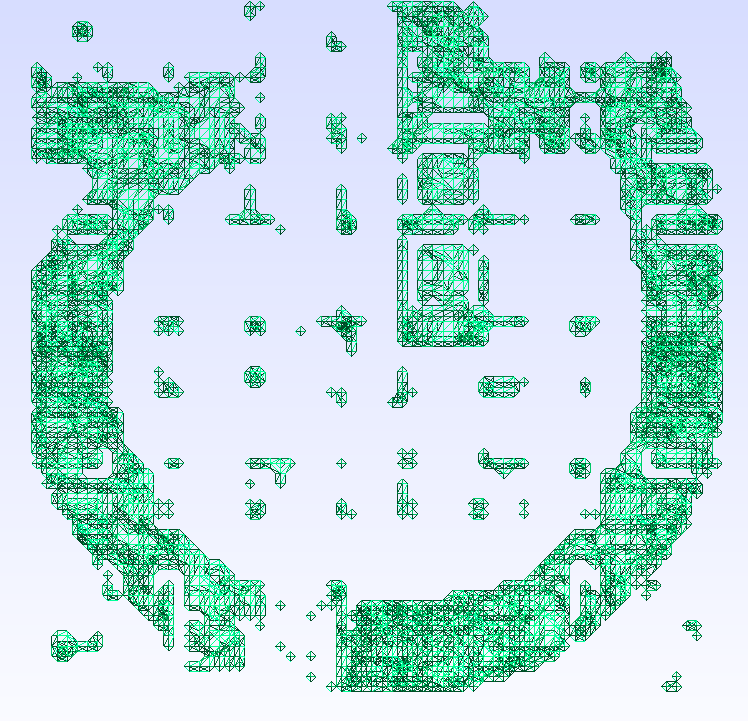
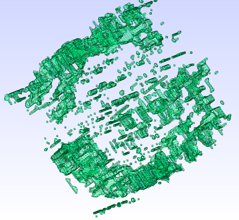
Lets Make a Mesh!
cur_cloud = sess.run(cloud)
import pandas as pd
pd.DataFrame({"x":cur_cloud[:, 0], "y":cur_cloud[:, 1], "z":cur_cloud[:, 2]}).to_csv("geb_1.csv")
#python ~/workspace/molten/cloud2mesh.py geb_1.csv --output geb_1.stl
#gmsh geb_1.stl
Hints of G
Not Quite Perfect
Print It !
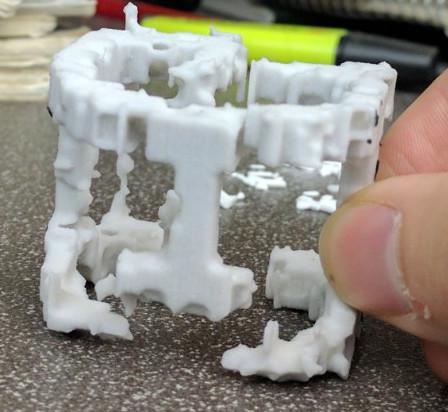
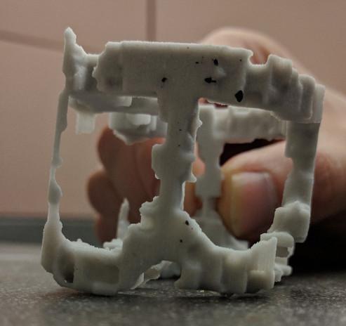
!python ~/workspace/molten/molten.py --help
An Physical Model of Common Machine Learning Woes!
%%HTML
<video width="640" height="480" controls>
<source src="../videos/geb-lrate05.mp4" type="video/mp4">
</video>
- Highly Non-Linear
- Millions of Local Optima
- Vanishing Gradients
- "Dead" parameters
- Imperfect metric
A Little More Complex
%%HTML
<video width="640" height="480" controls>
<source src="../videos/logo1.mp4" type="video/mp4">
</video>
%%HTML
<video width="640" height="480" controls>
<source src="../videos/logo-lrate05.mp4" type="video/mp4">
</video>
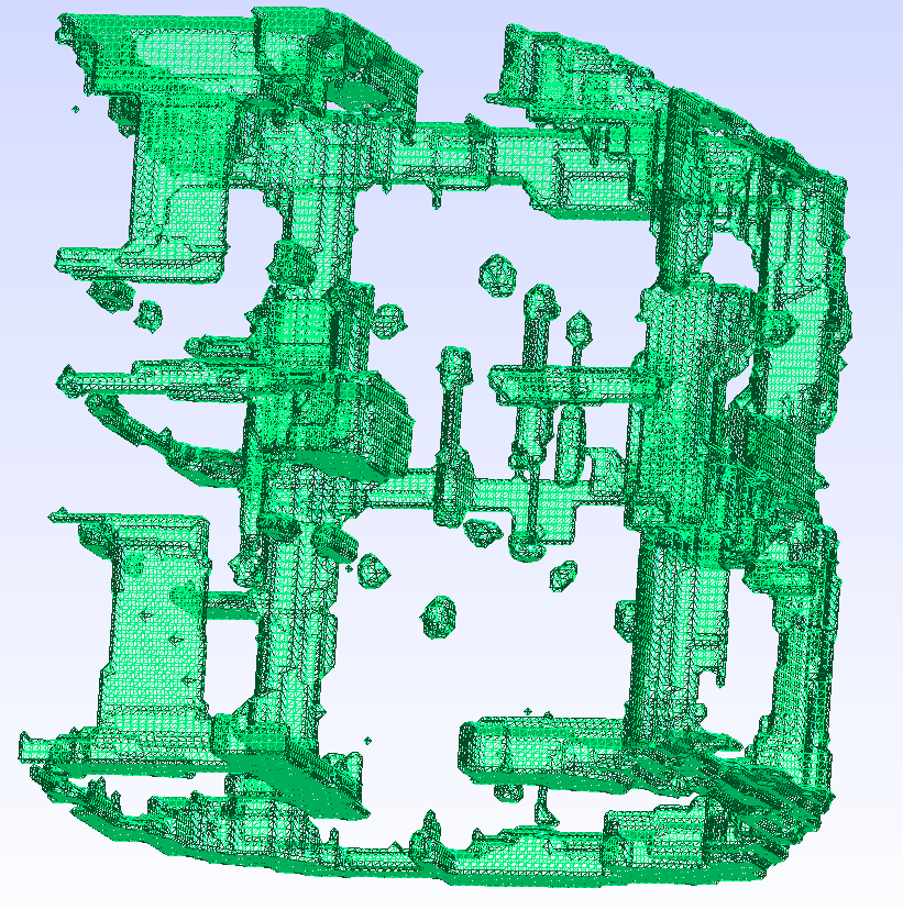
Tools For Defeating Machine Learning Dragons
- Regularization Losses
- Dropout
- Data Augmentation
- Early Stopping
- Simulated Annealing
- Mini-Batches
- Momentum
Comments
Comments powered by Disqus